High Performance Computing
Five projects that build on each other, from tuning C code on one CPU to running a galaxy simulation on four GPUs at once.
9.5Course grade
N-body on GPUs
2,910× faster than the single-core version


A galaxy simulation: every body pulls on every other body, every step. We started from a plain single-core C program and made it faster one change at a time, ending on four NVIDIA Tesla K80 GPUs working together.
- 2,910×faster than the single-core C version
- 431billion body-to-body interactions per second, up from 0.148
- 40×faster than our OpenMP version on the CPU
- 4NVIDIA Tesla K80 GPUs working at once
CLAHE
Contrast enhancement on GPU
What it is
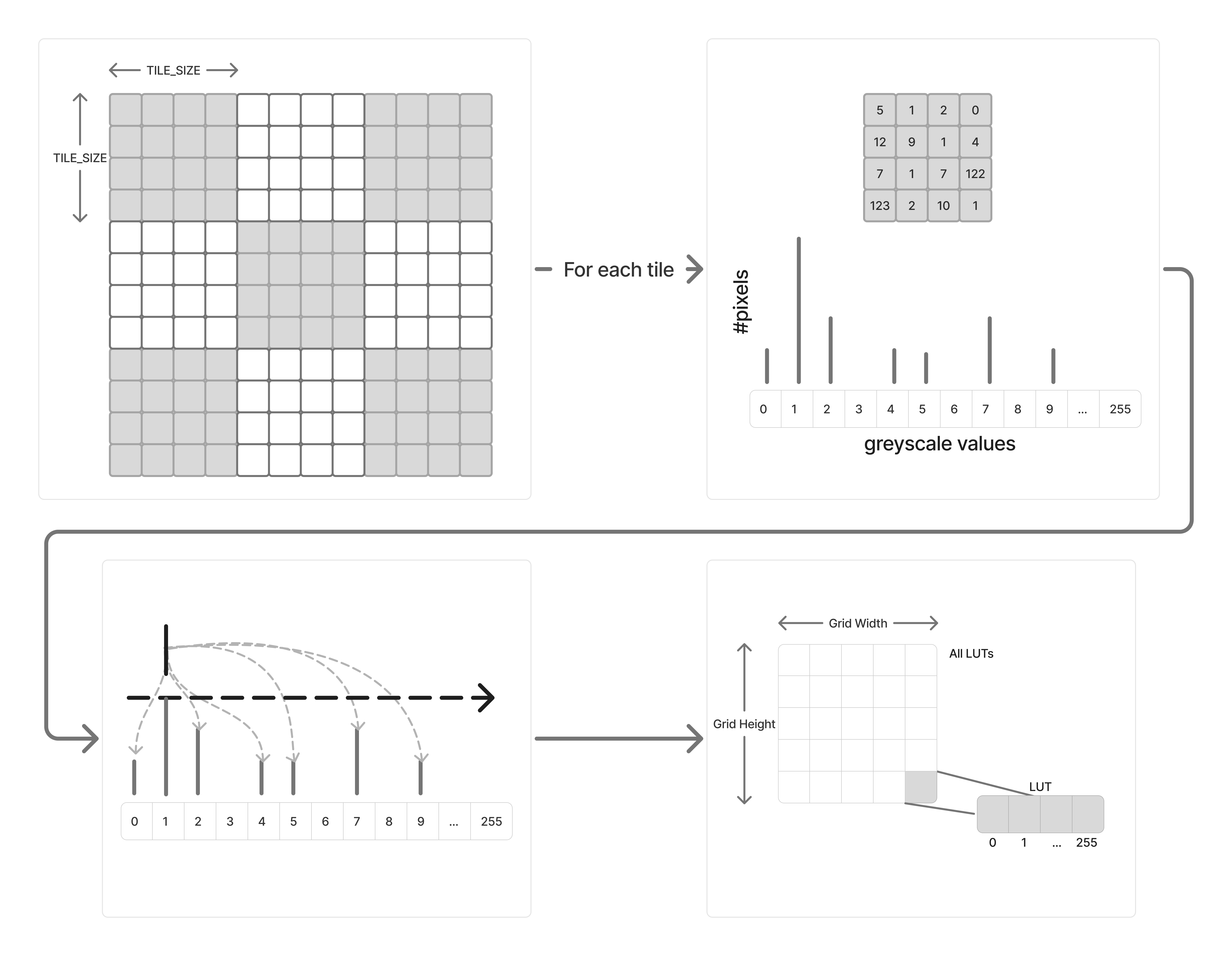
CLAHE (contrast-limited adaptive histogram equalisation) brings out detail in an image by evening out its contrast tile by tile, with a limit on how far it stretches any one tile. We moved it to an NVIDIA Tesla K80 GPU and made it faster one change at a time, measuring throughput in megapixels per second.
The final version runs at 1,333.8 MPixel/s, about 24× the CPU version’s 55.8.
The two steps
First, every tile counts how many of its pixels have each of the 256 grey levels, cuts every count above a limit, spreads the excess evenly over all the levels, and turns the counts into a lookup table of running totals. Then every pixel’s new value is a blend of the lookup tables of its four nearest tiles.
Fewer kernels isn’t always faster
The first GPU version used three kernels: histograms, lookup tables, then the final pixels. Merging the first two, so the histograms never leave the GPU’s fast memory, made it slower: 470.1 against 703.5 MPixel/s. Each block had 1024 threads, one per pixel, but only 256 of them had work in the lookup-table half, and the rest sat idle while still holding their place on the multiprocessor.
Blocks of 256 threads, each counting four pixels, fixed that: 722.9.
Private histograms and a parallel scan
Threads adding to the same count with atomicAdd have to wait their turn. Each block now keeps 8 private copies of its histogram in shared memory, each used by a different group of threads, and adds them up at the end: 854.9.
The running totals for the lookup table became a parallel scan in shared memory, where the distance between the values each thread adds doubles at every step: 897.6.
Overlapping copies with work
The profiler showed most of the time going on copying the image to and from the GPU, not on the kernels. CUDA streams split the image into parts, so one part is copied while another is processed; about 8 streams worked best: 1,234.4.
Events then replaced the wait for the whole GPU between the two steps: each part starts as soon as the parts it needs are done, reaching 1,333.8.
Results
Throughput on a Tesla K80 in MPixel/s, after each change, on the same test image. Each version ran 25 times, leaving out the two extremes.
Code
//! Add histogram values to seperate private histograms
//* Indexing increased by blockDim (here is 16) 1 pixel for each quadrant
for (int cur_y = ty; cur_y < TILE_SIZE; cur_y += step_y) {
    for (int cur_x = tx; cur_x < TILE_SIZE; cur_x += step_x) {
        const int gx = x_start + cur_x;
        const int gy = y_start + cur_y;

        if (gx < w && gy < h) {
            const unsigned char pix = data[gy * w + gx];

            //! 1/<NUM_BANKS>th of the serialization
            atomicAdd(&(p_hist[bank_id][pix]), 1);
        }
    }
}
__syncthreads();

//! Sum the banks into the final result
int bin_sum = 0;
#pragma unroll
for (int k = 0; k < NUM_BANKS; k++) {
    bin_sum += p_hist[k][tid];
}
hist[tid] = bin_sum;CUDA convolution
Image filters on GPU
What it is
A 2D convolution slides a filter over an image, the basis of blurring, sharpening and edge detection. Ours runs in two passes, along the rows and then down the columns. We moved it to one NVIDIA Tesla K80 GPU on the course server, then measured how it scales against the CPU, from tiny images up to 16384×16384, and how far its answers drift from the CPU’s.
One thread per pixel
A first version used a single block of 1024 threads, one per pixel, so it could only handle a 32×32 image; anything bigger stopped with an “invalid argument” error. The real version uses a grid of 32×32-thread blocks, and each thread works out which pixel is its own from its block and thread numbers.
Memory sets the limit
In theory the grid of blocks covers images far bigger than any GPU could hold; in practice the GPU’s memory runs out first. With the input, a buffer and the output each the size of the image, the largest square image is 31618 pixels a side. Writing the result over the input array instead raised it to 38725.
Float or double
The GPU fuses a multiply and an add into one instruction with a single rounding; the CPU rounds after each step. In single precision the answers drift apart as the filter grows, from 0.0078125 at a radius of 1 to 640 at a radius of 256. In double precision the gap stays around a millionth even at 256.
Doubles cost speed, though: at 8192×8192 the GPU’s lead drops from 16.97× to 14.45×.
No divergence at the edges
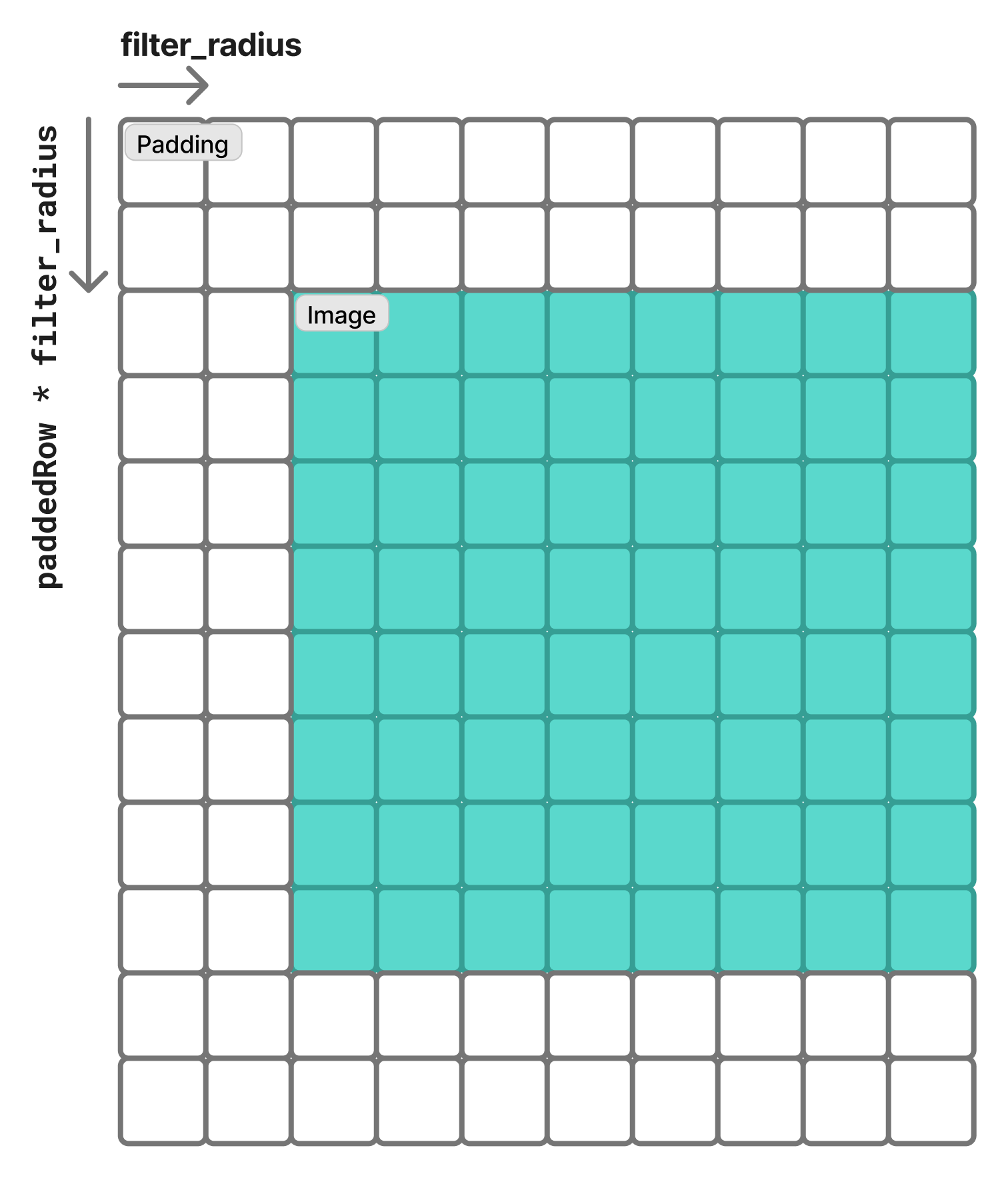
Pixels near the edge need bounds checks the others don’t, so the threads of one warp take different paths and wait for each other. A border of padding as wide as the filter’s radius removes the checks.
On the K80 the gain was cancelled out by the more complex copies of the padded image. On an RTX 3060 with a 16384×16384 image, the padded version was faster at every filter size: 0.99 to 0.92 seconds at a radius of 128, and 13.05 to 10.91 at 4096.
Results
How many times faster the GPU is than the CPU, single precision, by image size.
Code
__global__ void convolutionRowGPU(PixelScalar *d_Dst, PixelScalar *d_Src, PixelScalar *d_Filter,
                               int imageW, int imageH, int filterR) {
    int k;
    PixelScalar sum = 0;
    int paddedWidth = (imageW + filterR);
    int x = blockIdx.x * blockDim.x + threadIdx.x + filterR;
    int y = blockIdx.y * blockDim.y + threadIdx.y + filterR;

    for (k = -filterR; k <= filterR; k++) {
        int d = x + k;

        sum += d_Src[y * paddedWidth + d] * d_Filter[filterR - k];
    }

    d_Dst[y * paddedWidth + x] = sum;
}K-means
Clustering on 56 threads
What it is
K-means sorts points into k groups: each point joins its nearest centre, each centre moves to the average of its points, and the two steps repeat until the groups stop changing, or for at most 500 rounds. We parallelised the course’s sequential C version with OpenMP on the course server, an Intel Xeon E5-2695 v3 machine with 56 threads.
Where the parallel work is
The rounds can’t run in parallel: each one needs the centres from the round before. Inside a round, though, every point finds its nearest centre on its own, so one #pragma omp parallel for shares the points out across the threads. The second loop, which turns the sums into new centres, has no dependencies either and gets the same treatment.
SIMD for the distances
Intel VTune showed most of the time going into the function that measures the distance from a point to a centre. Splitting it across threads made it slower: each call has too little work. Instead, #pragma omp simd turns its loop into vector instructions, and the Xeon’s AVX2 does 8 float operations at once.
What didn’t work
We also tried threads inside the nearest-centre search, with a hand-written minimum, since the OpenMP version we had couldn’t reduce arrays. It was slower than the sequential code. Nesting, with 14 threads over the points and 3 inside the search, did no better: starting and managing the extra threads cost more than they saved.
Results
Speed against the sequential version on the course server, by thread count and by how the threads add to the shared sums.
Code
delta = 0.0;
#pragma omp parallel for private(j, index) reduction(+:delta)
for (i=0; i<numObjs; i++) {
    /* find the array index of nestest cluster center */
    index = find_nearest_cluster(numClusters, numCoords, objects[i],
                                 clusters);

    /* if membership changes, increase delta by 1 */
    if (membership[i] != index) delta += 1.0;

    /* assign the membership to object i */
    membership[i] = index;

    /* update new cluster center : sum of objects located within */
    #pragma omp atomic
    newClusterSize[index]++;

    for (j=0; j<numCoords; j++) {
        #pragma omp atomic
        newClusters[index][j] += objects[i][j];
    }
}Sobel filter
Image edges, 21× faster
What it is
A Sobel filter finds the edges in an image: for every pixel it weighs the eight pixels around it twice, once for change across and once for change down, and combines the two. We started from the course’s plain C version and made it as fast as we could on a single core of an Intel Core i5-1235U, measuring every change on a 4096×4096 image.
No threads and no GPU in this one: only the way the code reads memory and does its maths. Every change was timed with the compiler’s optimisations off (-O0) and at its fastest setting (-fast), because a change that helps one can do nothing, or harm, at the other.
Reading memory in order
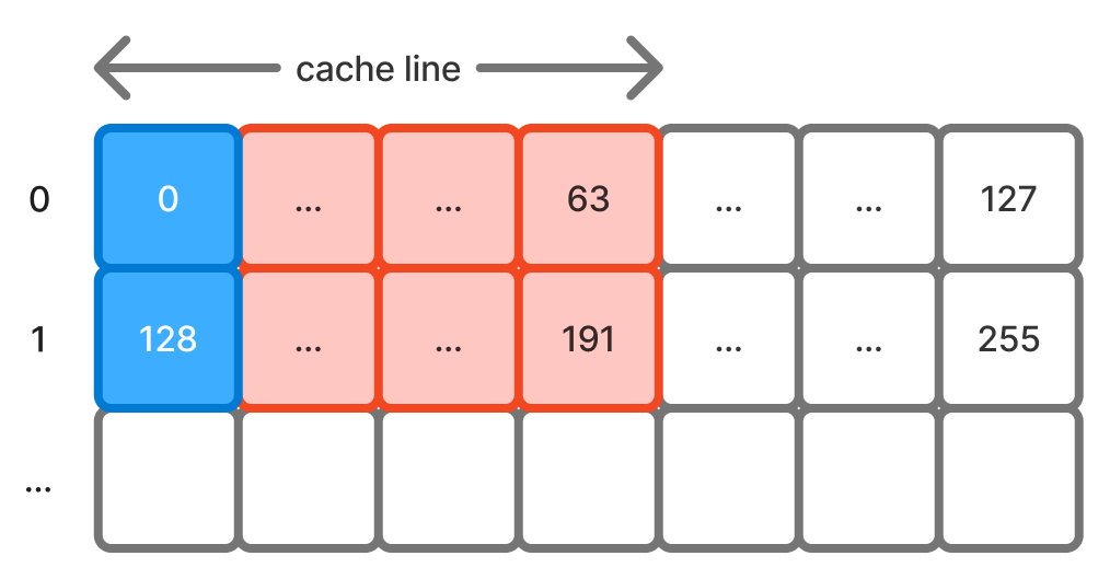
The original loops walked down each column. Every read pulls a whole cache line into the processor’s cache, but a walk down a column uses one value from that line and moves on to the next row, so the rest is thrown out before it’s ever used.
Swapping the two loops so they walk along rows cut cache misses from 57.7M to 2.6M (22×) with optimisations off, and on its own made the fastest build 2.79× faster.
Less work per pixel
Then the classic changes, one at a time. Unrolling handles four pixels per pass of the inner loop, so the loop counts and checks a quarter as often. The convolution function became inline code instead of a call. Squares became multiplications instead of calls to pow(). Together they reached 5.02×.
Not every textbook change helped. Working out repeated expressions once, outside the loop, made the fastest build slightly slower (4.38× to 4.12×): the compiler already did it, and better. Later, once the maths got cheap, the program was limited by memory instead, so the final versions drop the unrolling and the merged error check that read a second image in the same loop.
Simpler maths
The Sobel filter’s weights are only 1 and 2, so each convolution becomes additions, subtractions and shifts, worked out one row of the filter at a time so the reads follow memory. This one change took the fastest build from 6.11× to 17.30×.
A faster square root
Each output pixel needs a square root. Like the fast inverse square root trick, ours reads the floating-point number’s bits as an integer, halves it and adds a constant: one shift and one addition. The approximation comes from treating log₂(1 + x) as x + 0.043.
Two other tricks, a branch-free min() and a rearranged error check, made the fastest build slower (13.18× and 11.69×), so the final version keeps only the fast convolution and the fast square root: 21.49×.
Results
Speed against the original C code on one core of an Intel Core i5-1235U, 4096×4096 image, Intel compiler at its fastest setting. Each version ran 12 times; the average leaves out the fastest and the slowest run.
Code
for (i = 1; i < SIZE - 1; i++) {
    // Referencing
    const unsigned char *top_row = &input[dec_i_times_SIZE];
    const unsigned char *bottom_row = &input[inc_i_times_SIZE];
    const unsigned char *mid_row = &input[i_times_SIZE];
    unsigned char *out_row = &output[i_times_SIZE];

    for (j = 1; j < SIZE - 1; j++) {
        pixel_horizontal = -top_row[j - 1] + top_row[j + 1];
        pixel_vertical = top_row[j - 1] + (top_row[j] << 1) + top_row[j + 1];
        pixel_horizontal += -(mid_row[j - 1] << 1) + (mid_row[j + 1] << 1) - bottom_row[j - 1] + bottom_row[j + 1];
        pixel_vertical += -bottom_row[j - 1] - (bottom_row[j] << 1) - bottom_row[j + 1];

        square_sum = pixel_horizontal * pixel_horizontal + pixel_vertical * pixel_vertical;
        sqrt = * ( int * ) &square_sum;
        sqrt = (sqrt >> 1) + 0x1FBD3F7D;
        res = (int) (* ( float * ) &sqrt);
        out_row[j] = (res > 255) ? 255 : (unsigned char)res;
    }
    dec_i_times_SIZE += SIZE;
    inc_i_times_SIZE += SIZE;
    i_times_SIZE += SIZE;
}Tools
What this course's projects were built with. Pick one to see where else I used it.